How to Use OMEGAlpes
OMEGAlpes stands for Generation of Optimization Models As Linear Programming for Energy Systems. It is an Open Source energy systems modelling tool for linear optimisation (LP, MILP).
They are using a specified graph representation described here: OMEGAlpes Representation
Examples
Please have a look to the following examples:
Example 1: PV self-consumption
In this PV self-consuption example, a single-house with roof-integrated photovoltaic panels (PV) is studied. Specifically, the study case is about demand-side management in order to maximize the self-consumption, by shifting two household appliances consumption (clothes washing machine and clothes dryer) and using a water tank for the domestic hot water consumption.
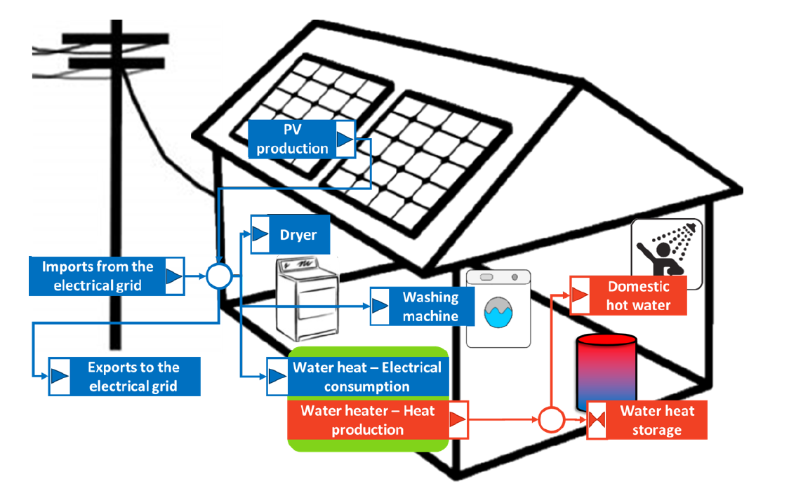
Figure 1: Principle diagram of the PV self-consumption example | Author: Camille Pajot
- This example leads to a study with :
6922 variables (2890 continuous and 4032 binary)
79172 non-zeros
This optimization problem has been generated within 1.2 seconds on an Intel bicore i5 2.4 GHz CPU.
An optimal solution was found in 43.6 seconds with the free CBC solver available in the PuLP package, and in the 2.5s with the commercial Gurobi solver.
Example 2: Waste heat recovery
In the waste_heat_recovery module, an electro-intensive industrial process consumes electricity and rejects heat. This waste heat is recovered by a system composed of a heat pump in order to increase the heat temperature, and a thermal storage that is used to recover more energy and have a more constant use of the heat pump. This way, the waste heat is whether recovered or dissipated depending on the waste heat recovery system sizing. The heat is then injected on a district heat network to provide energy to a district heat load. A production unit of the district heat network provides the extra heat.
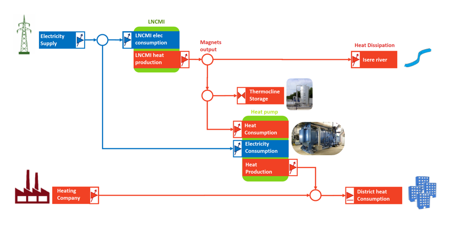
Figure 4: principle diagram of the waste heat recovery example | Author : Camille Pajot
Technical and decision constraints and objectives can be added to the project. This leads to the following Figure 5.
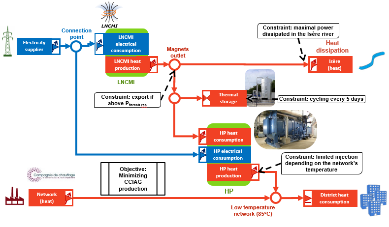
Figure 6: principle diagram of the waste heat recovery example with constraints | Author: Camille Pajot
Applying, multi-stakeholder vision on the waste heat recovery project leads to the Figure 6. One central point is the governance of the storage and heat pump. Who’s financing it? which actor will operate it? This governance needs to be discuss and mutually agreed to be able to go further on the project.
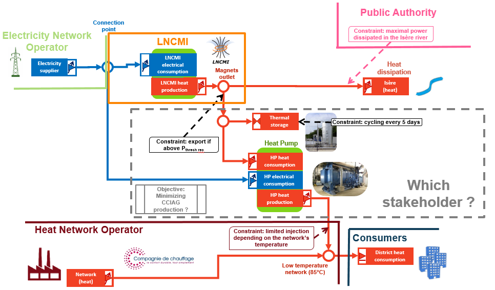
Figure 6: principle diagram of the waste heat recovery example with multi-stakeholder vision | Author: Lou Morriet from Camille Pajot work
- A technical optimisation over one year on a hourly time step can lead to a study with
228k variables (158k continuous et 70k binaires)
316k constraints
It has been solved in 13h with Gurobi, which can be considered as correct considering the high number of variables and constraints.
Considering the 20MWh / 6.7MW storage this can of study can calculate that 60% of the annual needs could be covered by the LNCMI waste heat (which corresponds to 60% reduction in CO2 emissions) /!This outputs should be consider regarding the constraints and objectives of the model, which are not totally detailed here, as the goal of this part is to show the possibilities of OMEGAlpes.
Graphics like the following one can also be produced:
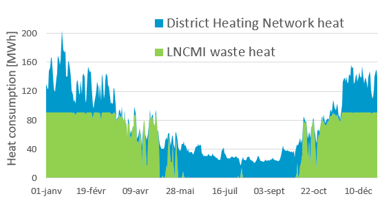
Figure 7: heat provider of the district over a year | Author: Camille Pajot
- Various studies could be carried out:
Balancing between CO2 emissions from the LNCMI and district heating, free profile
Using HP according to the electricity price, typical profiles
Study of operational performances under constraints, fixed profile
Example 3: Optimal Scheduling of Residential Heat Pumps at district level
In the residential heat pump (HP) optimal scheduling module, a methodology for managing the collective operation of heat pumps at the district level is presented. The approach optimizes schedules to minimize electrical energy consumption while maintaining occupant comfort and respecting grid operational limitations. Unlike strategies based on predetermined operational rules, this method uses automatically generated Mixed-Integer Linear Programming (MILP) models. The framework utilizes OMEGAlpes, which is coupled with a reduced-order Resistance-Capacitance (RC) thermal model to balance physical accuracy with computational tractability. Furthermore, it integrates internal heat gains and temperature setpoints derived from the RichardsonFR model, which leverages occupant behavior and appliance usage data to improve load estimation accuracy.
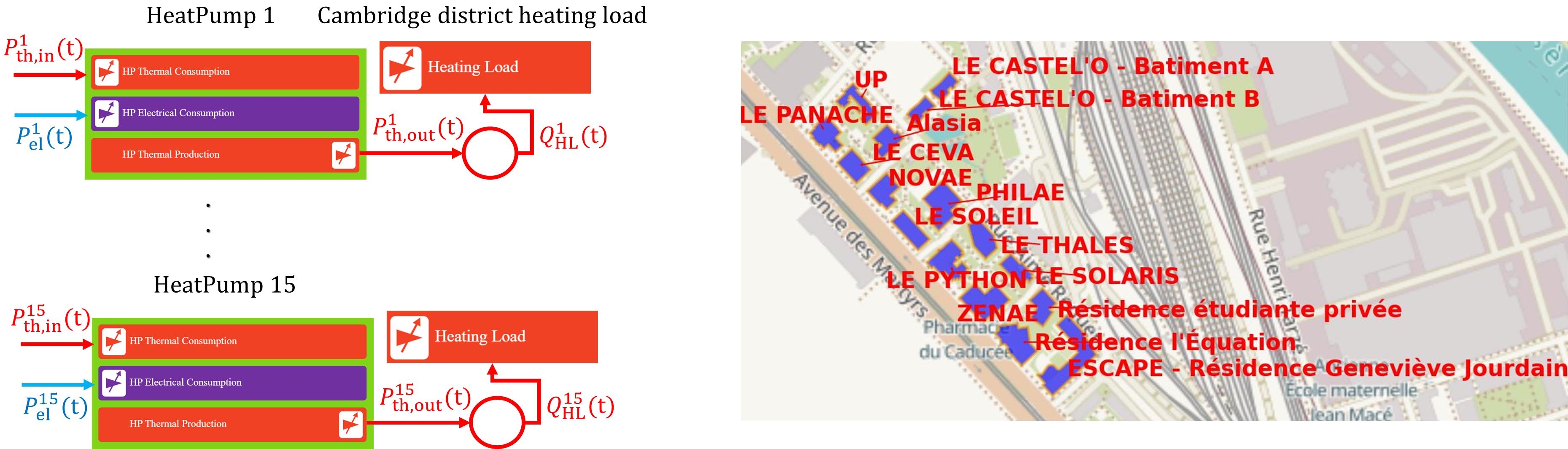
Figure 1: Principle diagram of the residential district heat pump control example | Author: Mainak Dan
The framework compares two control strategies—decentralized and coordinated—across a cluster of 15 residential buildings in Grenoble.
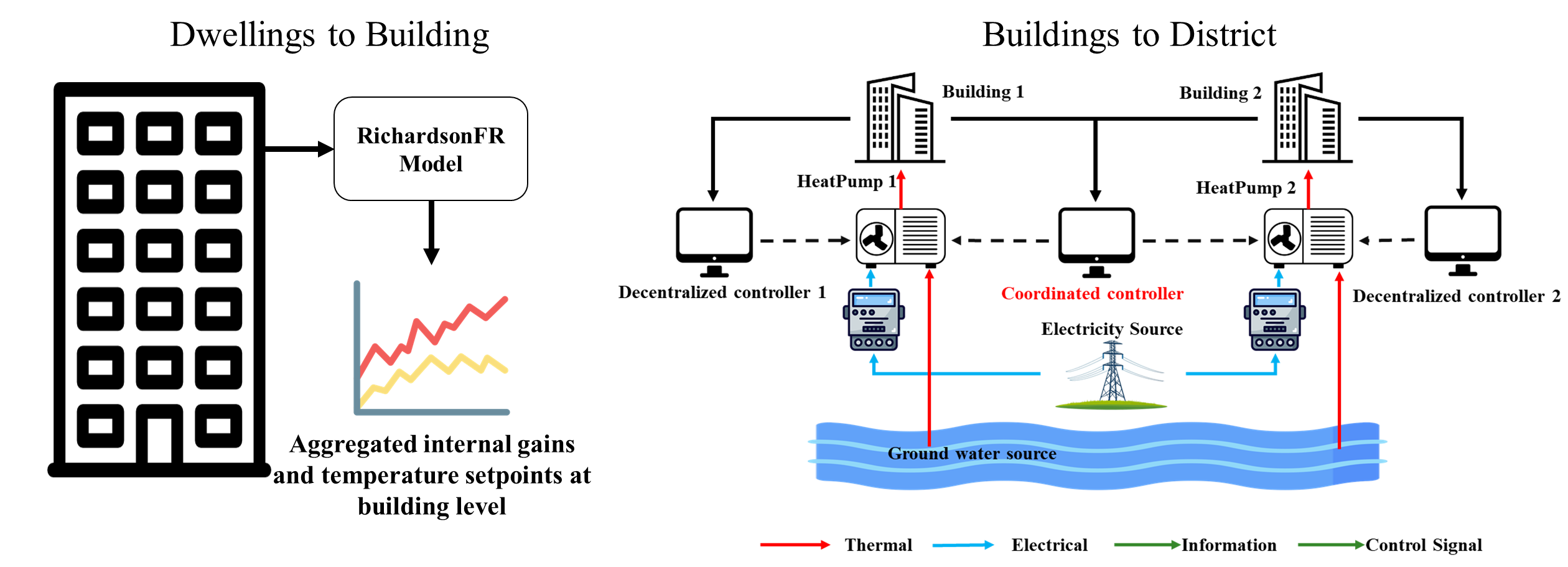
Figure 2: Principle diagram of decentralized vs. coordinated HP control strategies | Author: Mainak Dan
- A technical optimization over a representative winter month at a 10-minute time step results in a study with:
~1.7 million variables
~2 million constraints
It was solved using Gurobi with an optimality gap of 0.005, with solution times of approximately 86.7 seconds for the decentralized case and 270.3 seconds for the coordinated case. The study demonstrates that coordinated control effectively leverages building thermal mass to manage grid stress, achieving significant performance improvements:
31% reduction in maximum aggregated peak demand.
32% reduction in the peak-to-average power ratio.
These outputs should be considered regarding the specific constraints and objectives of the model, as the primary goal of this implementation is to demonstrate the flexibility and scalability of OMEGAlpes in district-level energy management. Graphics like the following can also be produced:
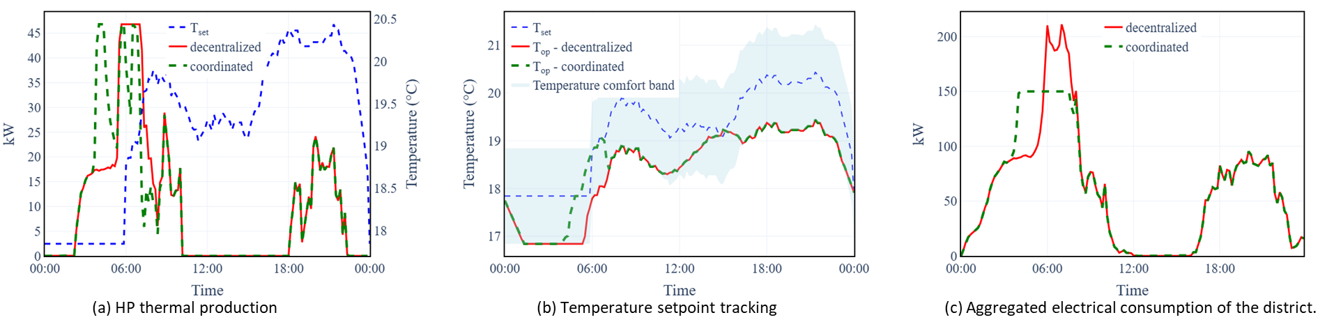
Figure 3: Collective electricity consumption and temperature setpoint tracking of the district over a representative period | Author: Mainak Dan
Various studies could be carried out using this framework:
Comparison of decentralized versus coordinated control strategies.
Impact of occupant behavior variability on thermal load requirements.
Sensitivity analysis of demand-side management under different grid power constraints.
Example 4: Adding Custom Constraints, Objective and Visualizing Results
This example demonstrates how to define a custom optimization model, and custom constraints (such as ramping), and utilize OMEGALPES plotting tools to visualize the results.
from omegalpes.energy.energy_nodes import EnergyNode
from omegalpes.energy.units.consumption_units import FixedConsumptionUnit
from omegalpes.energy.units.production_units import VariableProductionUnit, FixedProductionUnit
from omegalpes.energy.units.storage_units import StorageUnit
from omegalpes.general.optimisation.elements import *
from omegalpes.general.optimisation.model import OptimisationModel
from omegalpes.general.time import TimeUnit
from omegalpes.general.utils.plots import plot_node_energy_flows, plot_quantity, plot_quantity_bar, FigureOptions

# 1. Define Temporal Horizon
time_ = TimeUnit(periods=24, dt=1)

# 2. Define Components
load = FixedConsumptionUnit(time_, name="load", p=[4.0]*24)
pv = FixedProductionUnit(time_, name="pv", p=[0,0,0,0,0,0,1,2,3,4,5,5,5,4,3,2,1,0,0,0,0,0,0,0])
battery = StorageUnit(time_, name="battery", pc_max=2, pd_max=2, capacity=10, e_0=4)
gen = VariableProductionUnit(time_, name="gen", p_max=10)

# 3. Connect Units to Node
node = EnergyNode(time_, "elec_node", energy_type="Electrical")
node.connect_units(load, pv, battery, gen)

# 4. Add Custom Dynamic Constraints (e.g., Ramp Constraint)
# Ensures |P(t) - P(t-1)| <= 1 kW
    #:param exp_t (str): constraint expression time-dependant
    #:param t_range (str): time range defining when the constraint is set
    #:param name (str): name of the constraint
    #:param active (bool): is the constraint activated or deactivated
    #:param parent: unit containing the constraint

ramp_up = TechnicalDynamicConstraint(name='ramp_up', t_range='for t in time.I[1:]',
                                      exp_t='gen_p[t] - gen_p[t-1] <= 1', parent=gen)
ramp_down = TechnicalDynamicConstraint(name='ramp_down', t_range='for t in time.I[1:]',
                                       exp_t='gen_p[t-1] - gen_p[t] <= 1', parent=gen)
setattr(gen, "ramp_up", ramp_up)
setattr(gen, "ramp_down", ramp_down)

# 5. Add Custom Objective
obj = Objective(name='min_gen_prod', exp='lpSum(gen_p[t] for t in time.I)', parent=gen)
setattr(gen, "min_gen_prod", obj)

# 6. Initialize the optimziation model and add the nodes
model = OptimisationModel(time=time_, name="Example_Model")
model.add_nodes(node)


#7. solve the optimization problem
model.solve_and_update()

# 6. Plotting Results
# You can now choose between static or interactive plots
plot_node_energy_flows(node=node)
plot_quantity(time=time_, quantity=gen.p, interactive=False)
plot_quantity_bar(time=time_, quantity=battery.charge.p, interactive=False)
plot_quantity_bar(time=time_, quantity=battery.discharge.p, interactive=False)
plot_quantity_bar(time=time_, quantity=battery.e, interactive=False)
Key takeaways from this example:
Custom Constraints: Use TechnicalDynamicConstraint to define temporal dependencies within your unit operations.
Model Integration: Use setattr to attach objectives and constraints to existing model components.
Visualization: OMEGAlpes provides high-level plotting functions to quickly assess energy balances and unit behaviors.
Example 5: Custom Prosumer Implementation
This example demonstrates how to create a scalable CustomProsumer class in OMEGAlpes that dynamically attaches energy units to a local node based on configuration dictionaries[cite: 1].
Class Definition
The following class wraps the Prosumer actor, automating the creation and connection of energy units.
from omegalpes.general.time import TimeUnit
from omegalpes.general.optimisation.model import OptimisationModel
from omegalpes.energy.energy_nodes import EnergyNode
from omegalpes.energy.units.consumption_units import FixedConsumptionUnit, ShiftableConsumptionUnit, VariableConsumptionUnit
from omegalpes.energy.units.production_units import FixedProductionUnit, VariableProductionUnit
from omegalpes.energy.units.storage_units import StorageUnit
from omegalpes.actor.operator_actors.prosumer_actors import Prosumer

class CustomProsumer:
    """
    A scalable wrapper class that creates a Prosumer's local node and dynamically
    attaches multiple energy units based on lists of configuration dictionaries.
    """
    def __init__(self, name, time,
                 fixed_loads=None, shiftable_loads=None, variable_loads=None,
                 fixed_productions=None, variable_productions=None,
                 storages=None):

        self.name = name
        self.time = time
        self.local_node = EnergyNode(name=f"{name}_local_node", time=time)

        self.consumption_units = []
        self.production_units = []
        self.storage_units = []

        fixed_loads = fixed_loads or []
        shiftable_loads = shiftable_loads or []
        variable_loads = variable_loads or []
        fixed_productions = fixed_productions or []
        variable_productions = variable_productions or []
        storages = storages or []

        # --- 1. Consumption Units ---
        for i, conf in enumerate(fixed_loads):
            unit_name = f"{name}_{conf.get('name', f'fixed_load_{i}')}"
            unit = FixedConsumptionUnit(time=time, name=unit_name, p=conf['p'])
            self.consumption_units.append(unit)

        for i, conf in enumerate(shiftable_loads):
            unit_name = f"{name}_{conf.get('name', f'shiftable_load_{i}')}"
            unit = ShiftableConsumptionUnit(time=time, name=unit_name, power_values=conf['power_values'])
            self.consumption_units.append(unit)

        for i, conf in enumerate(variable_loads):
            unit_name = f"{name}_{conf.get('name', f'variable_load_{i}')}"
            unit = VariableConsumptionUnit(time=time, name=unit_name,
                                           p_min=conf.get('p_min', 0), p_max=conf['p_max'])
            self.consumption_units.append(unit)

        # --- 2. Production Units ---
        for i, conf in enumerate(fixed_productions):
            unit_name = f"{name}_{conf.get('name', f'fixed_prod_{i}')}"
            unit = FixedProductionUnit(time=time, name=unit_name, p=conf['p'])
            self.production_units.append(unit)

        for i, conf in enumerate(variable_productions):
            unit_name = f"{name}_{conf.get('name', f'variable_prod_{i}')}"
            unit = VariableProductionUnit(time=time, name=unit_name,
                                          p_min=conf.get('p_min', 0), p_max=conf['p_max'])
            self.production_units.append(unit)

        # --- 3. Storage Units ---
        for i, conf in enumerate(storages):
            unit_name = f"{name}_{conf.get('name', f'storage_{i}')}"
            unit = StorageUnit(time=time, name=unit_name, capacity=conf['capacity'])
            self.storage_units.append(unit)

        # --- 4. Connect all gathered units ---
        all_units = self.consumption_units + self.production_units + self.storage_units
        if all_units:
            self.local_node.connect_units(*all_units)

        # --- 5. Instantiate OMEGAlpes Prosumer Actor ---
        self.actor = Prosumer(
            name=f"{name}_actor",
            operated_consumption_unit_list=self.consumption_units,
            operated_production_unit_list=self.production_units,
            operated_storage_unit_list=self.storage_units,
            operated_node_list=[self.local_node]
        )
Usage Example
Below is how you can use the class to define and instantiate multiple prosumers.
time = TimeUnit(periods=24, dt=1)
load_profile = [2, 2, 2, 2, 3, 4, 6, 5, 4, 3, 3, 3, 3, 3, 3, 4, 5, 7, 8, 6, 5, 4, 3, 2]
pv_profile = [0, 0, 0, 0, 0, 0, 2, 6, 10, 14, 16, 18, 18, 16, 14, 10, 6, 4, 0, 0, 0, 0, 0, 0]

prosumer_configs = [
    {
        "name": "P1",
        "fixed_loads": [{"name": "base_load", "p": load_profile}],
        "shiftable_loads": [{"name": "flex_load", "power_values": [2]}],
        "fixed_productions": [{"name": "pv_array", "p": pv_profile}],
        "storages": [{"name": "battery", "capacity": 10}],
        "objective": "maximize_selfconsumption_rate"
    }
]

for config in prosumer_configs:
    objective = config.pop("objective", None)
    p = CustomProsumer(time=time, **config)
    if objective == "maximize_selfconsumption_rate":
        p.actor.maximize_selfconsumption_rate(time=time)
How to Run an Example
The example codes are stored at the Gitlab: OMEGAlpes Examples in the folder “beginner_examples” or “examples”. Some of them have also been developed on a Jupyter notebook for a better understanding.
Note
To know how to run the example python codes or the notebooks, see: Help run Jupyter Notebook
Note
The examples may be updated with the last developer version which may be different from the OMEGAlpes user (Pypi) version. Thus, you may have to run the examples with the developer version. Otherwise you have to select the example version corresponding to the current Pypi version. The version used is indicated at the beginning of the example module.
In order to run example, you first need to download (or clone) the OMEGAlpes Examples folder (repository) at : OMEGAlpes Examples. In fact, it is better to download the whole folder as most of the examples or article case studies use data located outside the code file.
Then, open your development environment, select the example file you want (.py) and run it.
Note
Do not forget: To run your example, you first need to install OMEGAlpes library. To do so, please, have a look to the documentation: OMEGAlpes Installation Or to the README.md of OMEGAlpes Gitlab
Model Templates
This page is under development and wil be updated
OMEGAlpes use principles will be detailed here.
Please click on the following link to have a look to OMEGAlpes examples and study cases: OMEGAlpes Examples Documentation
In the meantime, empty templates for creating OMEGAlpes models including actors or not are available in this OMEGAlpes examples folder: Templates
A tutorial with linked notebooks are also available.
The notebook folder also enable to discover OMEGAlpes functionnalities, and especially this notebook about waste heat recovery.